Potato Late Blight – Part 2
Field assessment of potato late blight from UAV-based multispectral imagery
Part 2
Guide 2 of 2
Introduction
The first tutorial allowed us to train 5 models for classification: Random forest, Gradient Boost Classifier, Support Vector Classifier, Linear Support Vector Classifier, and K-Nearest Neighbours. Now we are going to use those models to classify a new dataset: May 26, 2018. Multispectral images of this dataset were acquired when late blight disease affected most of the potato crop.
Data and methods
The study area is a 1920 sq.m. potato field located in Subachoque, Colombia (see figure). This field is part of an experimental plot designed to evaluate the potato Diacol capiro variety response to different nutrient treatments. As the weather conditions favoured the appearance of late blight disease in several plots, the project had the chance to monitor the crop disease development. The experimental plot was inspected every seven days during the entire crop life span (i.e. 120 days from planting to maturity).
The generated mosaic covered an area of 3.2 Ha, which include the experimental plot and a bigger area where a different variety of potato was located, being this variety a yellow potato, this means, the tuber root colour it produces is yellow. In contrast, the potato from the experimental plot was from one variety of white potato (Diacol capiro). The experimental plot area was clipped by using a reference polygon (red polygon).
Study area:

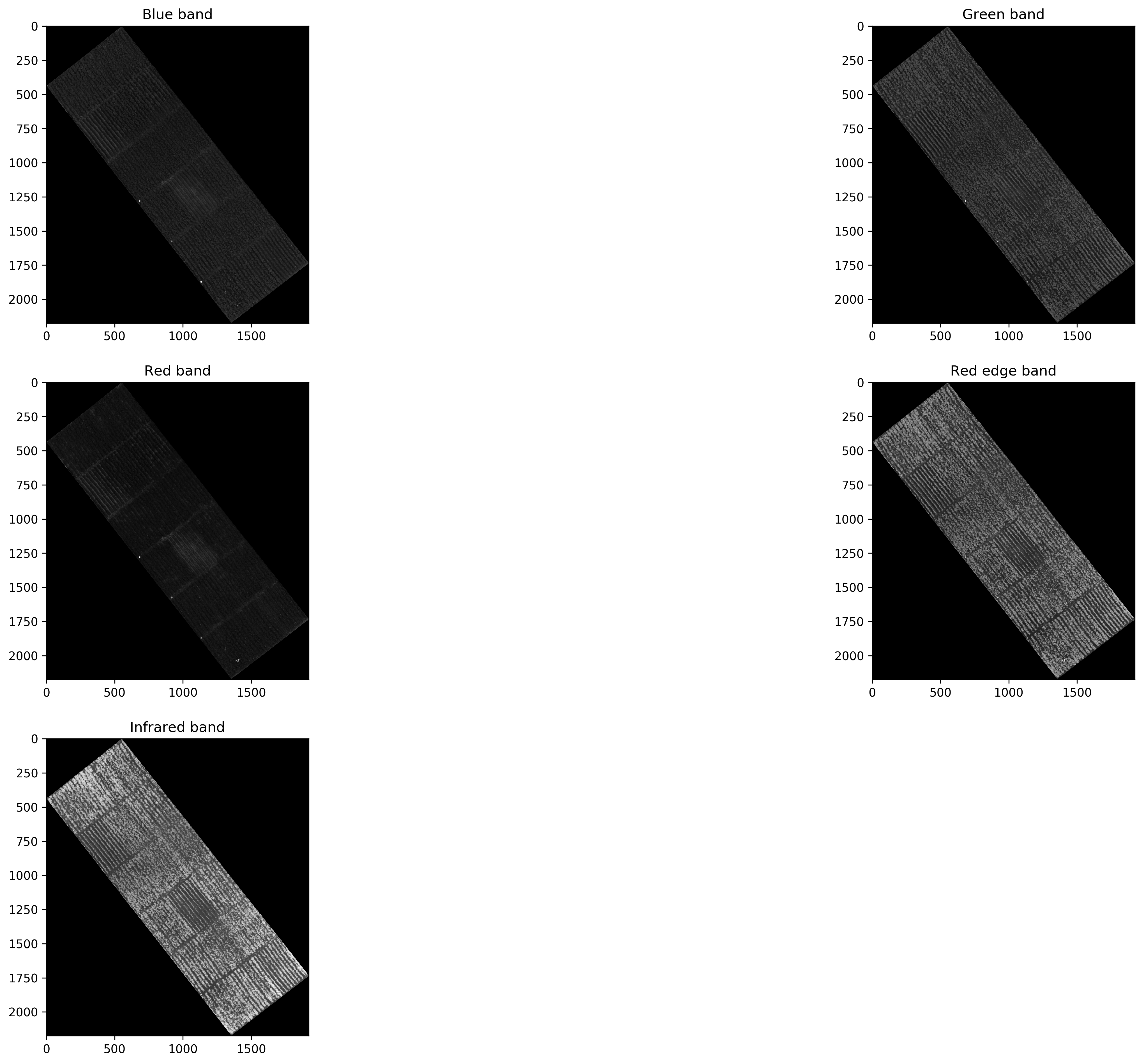
High resolution multispectral images were acquired at 40 m altitude above the ground surface at 11:00 am local time (GMT-5). Each multispectral image acquired by the MicaSense camera had five bands as described in the next table. In this work camera bands 4 and 5 have been reset according to the following order: Blue (B); Green (G); Red (R); Red edge (RE) and Near infrared (NIR).
| # Band | Name | Band center (nm) | Bandwidth FWHM (nm) |
|---|---|---|---|
| 1 | Blue | 475 | 20 |
| 2 | Green | 560 | 20 |
| 3 | Red | 668 | 10 |
| 4 | Near infrared |
840 | 40 |
| 5 | Red edge | 717 | 10 |
Experimental crop area consisted of an array of 18 blocks of 12 m $\times$ 8 m inside of a field of 77 m $\times$ 24 m. Each block had 9 rows arranged along the long side of the field with an area of 216 sq.m., the space between rows was 1m. Each row contained approximately 30 seed tubers of the same variety.
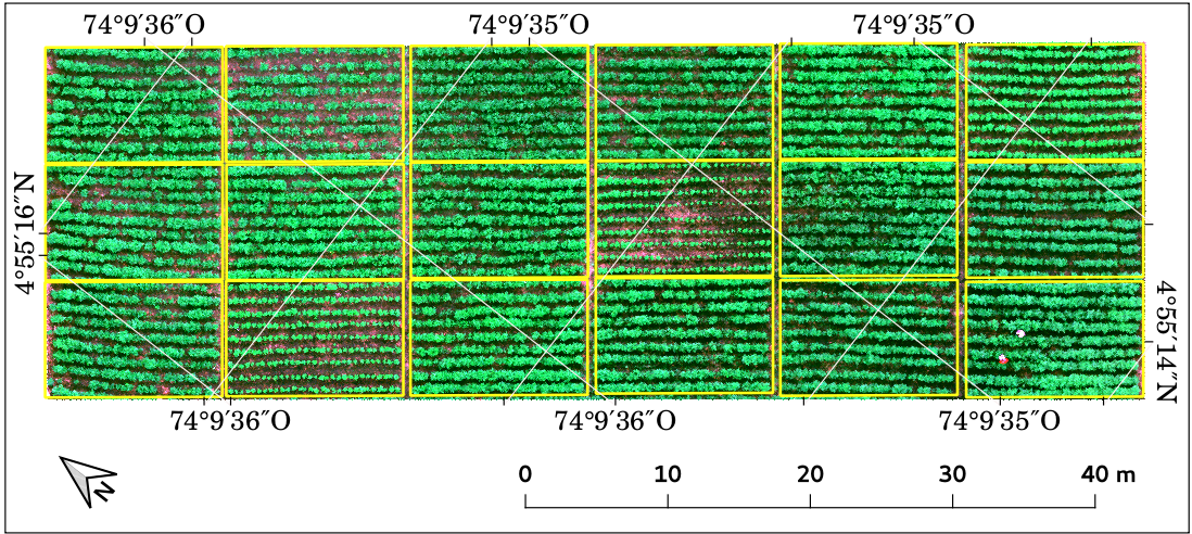 (a) May 12, 2018
 (b) May 26, 2018
The layout of the experimental crop. The yellow lines indicate the division of the field into 18 experimental blocks. (a) May 12, 2018; (b) May 26, 2018.
%matplotlib inline
import time
import os, shutil
from matplotlib import pyplot as plt
from matplotlib import colors
from IPython.display import Image
import numpy as np
import cv2
import math
import time
from osgeo import gdal
from skimage import img_as_ubyte
import scipy
import pandas as pd
from skimage.filters import threshold_otsu
import skimage.io as io

from sklearn.ensemble import AdaBoostClassifier, RandomForestClassifier, GradientBoostingClassifier, ExtraTreesClassifier
from sklearn.externals import joblib
from sklearn.metrics import plot_roc_curve, classification_report, confusion_matrix
from sklearn.model_selection import train_test_split

from sklearn.svm import SVC, LinearSVC
from sklearn.neighbors import KNeighborsClassifier
ds = gdal.Open('Raster/Correccion_reflectancia/MR_CE_20180526_Subachoque.tif')
# asignacion cada banda
AZUL = ds.GetRasterBand(1).ReadAsArray()
VERDE = ds.GetRasterBand(2).ReadAsArray()
ROJO = ds.GetRasterBand(3).ReadAsArray()
REDEDGE = ds.GetRasterBand(4).ReadAsArray()
NIR = ds.GetRasterBand(5).ReadAsArray()

srs = ds.GetProjectionRef()
geo_transform = ds.GetGeoTransform()

plt.figure(1, dpi=300)
plt.subplots_adjust(left=0.0, right=3.0, bottom=0.0, top=3.0)
plt.subplot(321) ,plt.imshow(AZUL, cmap='gray'),plt.title('Blue band')
plt.subplot(322) ,plt.imshow(VERDE, cmap='gray'),plt.title('Green band')
plt.subplot(323) ,plt.imshow(ROJO, cmap='gray'),plt.title('Red band')
plt.subplot(324) ,plt.imshow(REDEDGE, cmap='gray'),plt.title('Red edge band')
plt.subplot(325) ,plt.imshow(NIR, cmap='gray'),plt.title('Infrared band')
plt.show()
Thresholding
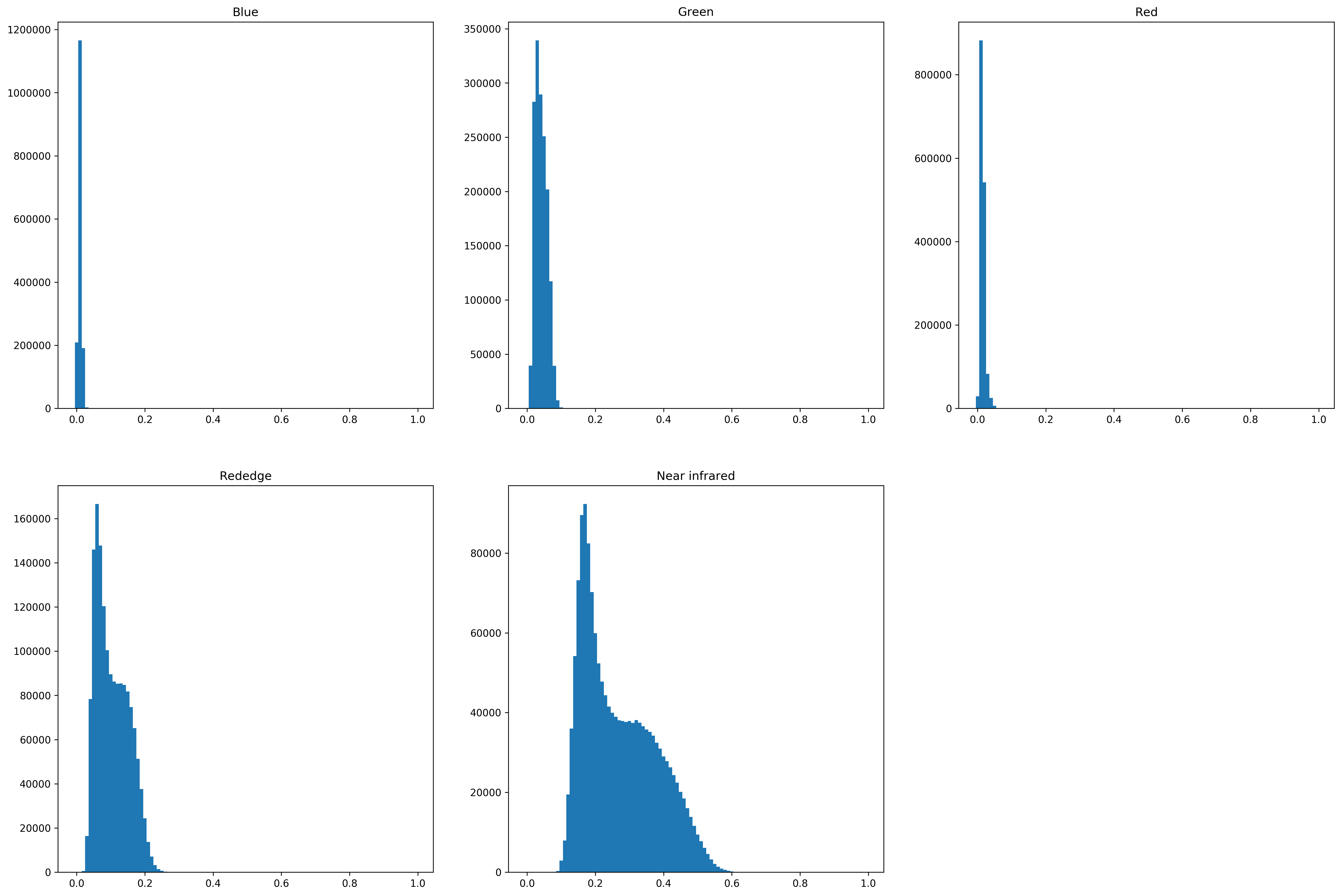
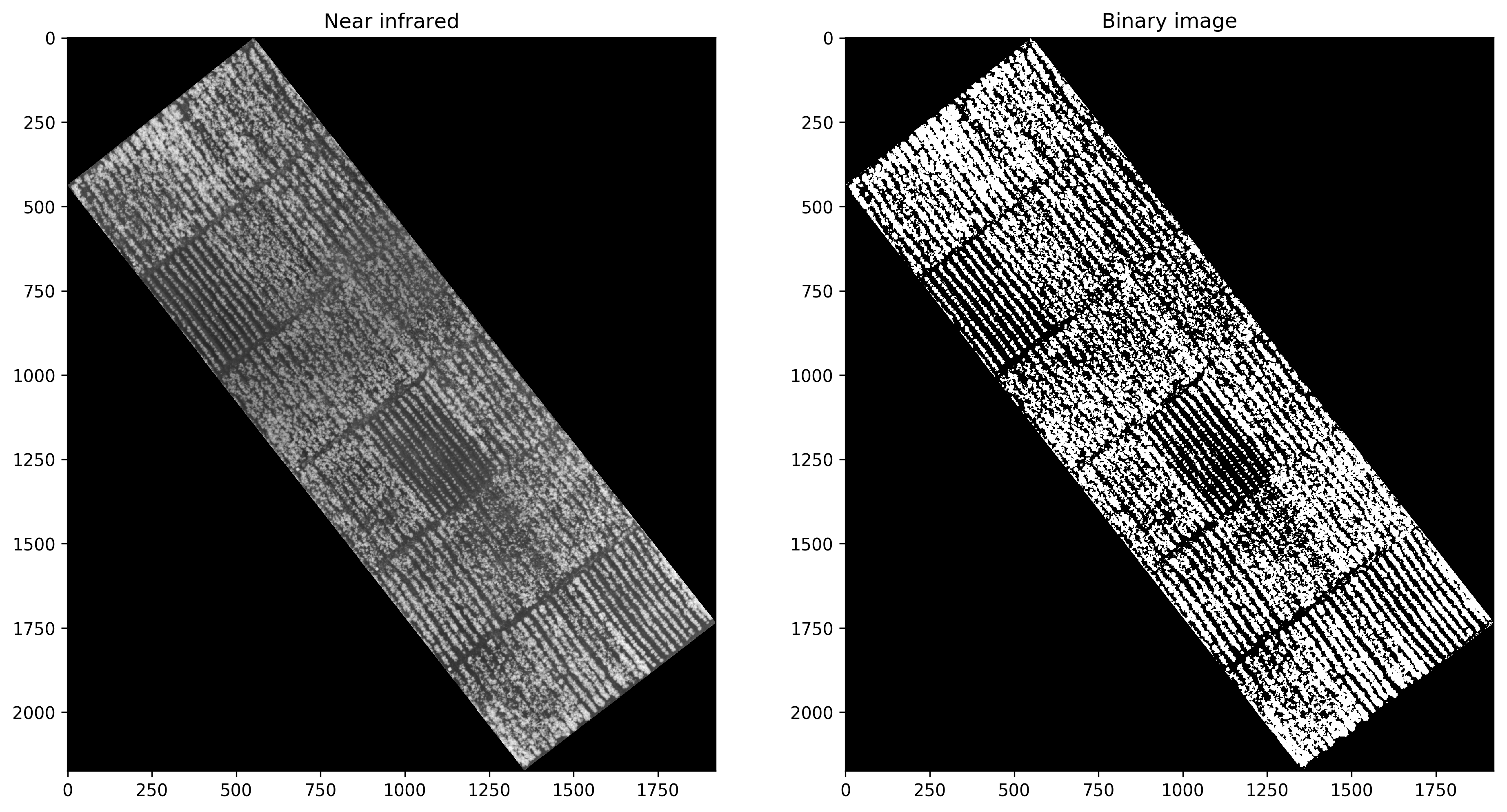
A thresholding technique reduces a grey-level image into an image where objects and background are represented with two levels: a binary image (Glasbey, 1993). Because of the difference in reflectance between the soil and the potato plants, both near infrared and red edge bands allowed separation of the potato plants from the soil.
The first step was to analyse multispectral bands of the orthomosaics by plotting their histograms. The next figure shows the histogram for each band in the multispectral orthomosaic for the two categories under study as well as ground reference images of the two categories. Green, Rededge and Near infrared bands have right-skewed bimodal histograms in the first category. Bands with high weed presence had a right-skewed histograms without a clear valley. Thresholding method used to separate vegetation was OTSU’s thresholding method (Otsu, 1979).
hist_b1 = np.histogram(AZUL[AZUL!=0].ravel(),100,[0,1])[0]
hist_b2 = np.histogram(VERDE[VERDE!=0].ravel(),100,[0,1])[0]
hist_b3 = np.histogram(ROJO[ROJO!=0].ravel(),100,[0,1])[0]
hist_b4 = np.histogram(REDEDGE[REDEDGE!=0].ravel(),100,[0,1])[0]
hist_b5 = np.histogram(NIR[NIR!=0].ravel(),100,[0,1])[0]

hist_range = np.arange(0,1,0.01)
plt.figure(1, dpi=300)
plt.subplots_adjust(left=0.0, right=3.0, bottom=0.0, top=3.0)
plt.subplot(231), plt.bar(hist_range,hist_b1,0.01), plt.title("Blue")
plt.subplot(232), plt.bar(hist_range,hist_b2,0.01),plt.title('Green')
plt.subplot(233), plt.bar(hist_range,hist_b3,0.01),plt.title('Red')
plt.subplot(234), plt.bar(hist_range,hist_b4,0.01),plt.title('Rededge')
plt.subplot(235), plt.bar(hist_range,hist_b5,0.01),plt.title('Near infrared')
(<matplotlib.axes._subplots.AxesSubplot at 0x7f2c0809df98>,
 <Container object of 100 artists>,
 <matplotlib.text.Text at 0x7f2c0e8f4ef0>)
image=REDEDGE
hist_image = image.ravel()
hist = np.histogram(image[image!=0].ravel(),100,[0,1])[0]
thresh = threshold_otsu(image)
thresh = thresh + 0.03
binary = image > thresh

plt.figure(1, dpi=300)
plt.subplots_adjust(left=0.0, right=3.0, bottom=0.0, top=3.0)
plt.subplot(131) ,plt.imshow(NIR, cmap='gray'),plt.title('Near infrared')
plt.subplot(132) ,plt.imshow(binary,cmap='gray'),plt.title('Binary image')
plt.show()

plt.show()
Masking image
To delete background from original multispectral image we multiply each band for the binary image resulting from thresholding step using the next equation:
where $C_{i}(x,y)$ is the resulting pixel at position $(x,y)$ for $i$ band without background, $A_{i}(x,y)$ is the original pixel at position $(x,y)$ for $i$ band of the multispectral image and $B(x,y)$ is the binary image pixel at position $(x,y)$ created in the thresholding process.
mask = np.array(binary, dtype='uint8')
filtered_mask = cv2.medianBlur(mask,3)

plt.figure(1, dpi=300)
plt.subplots_adjust(left=0.0, right=3.0, bottom=0.0, top=3.0)
plt.subplot(131) ,plt.imshow(NIR, cmap='gray'),plt.title('Banda NIR')
plt.subplot(132) ,plt.imshow(mask,cmap='gray'),plt.title('Mascara')
plt.subplot(133) ,plt.imshow(filtered_mask,cmap='gray'),plt.title('Mascara con filtro de mediana')
plt.show()

plt.show()
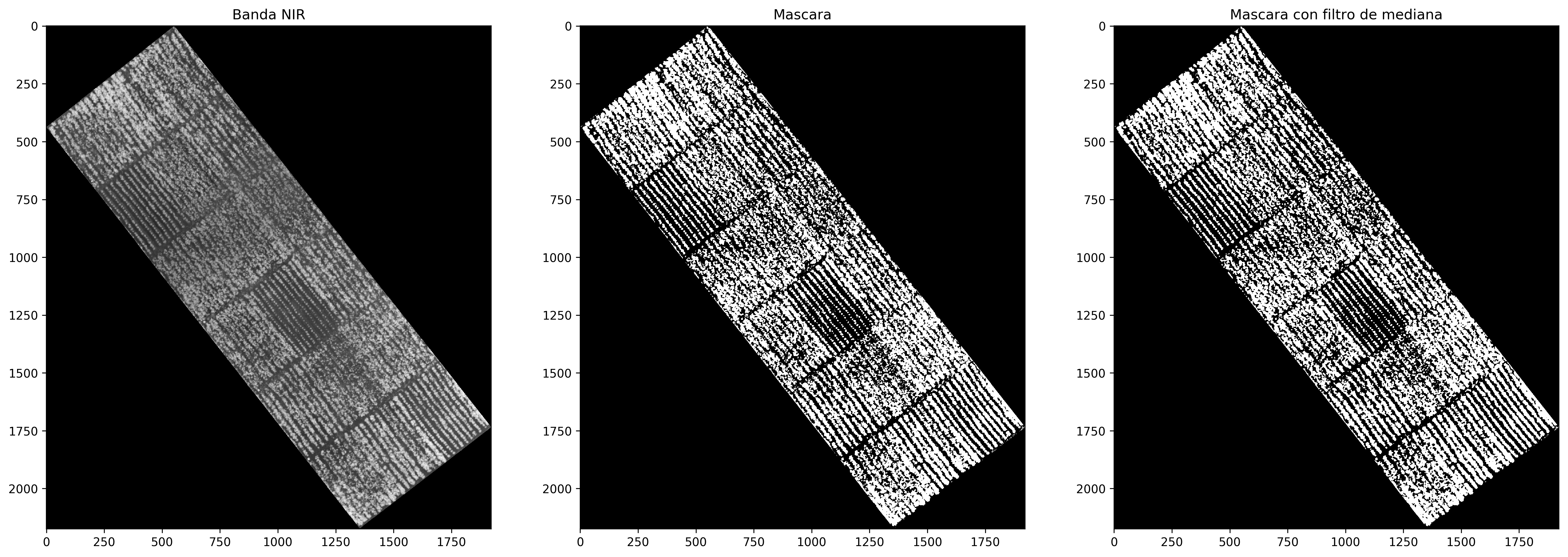
Here we can see how looks any band from the multispectral image after masking process. It can be seen how the ground surface does not appear any more.
azul_seg = AZUL*filtered_mask
verde_seg = VERDE*filtered_mask
rojo_seg = ROJO*filtered_mask
rededge_seg = REDEDGE*filtered_mask
nir_seg = NIR*filtered_mask

plt.figure(1, dpi=300)
plt.subplots_adjust(left=0.0, right=3.0, bottom=0.0, top=3.0)
plt.subplot(321) ,plt.imshow(azul_seg, cmap='gray'),plt.title('Blue')
plt.subplot(322) ,plt.imshow(verde_seg, cmap='gray'),plt.title('Green')
plt.subplot(323) ,plt.imshow(rojo_seg, cmap='gray'),plt.title('Red')
plt.subplot(324) ,plt.imshow(rededge_seg, cmap='gray'),plt.title('Red edge')
plt.subplot(325) ,plt.imshow(nir_seg, cmap='gray'),plt.title('Near infrared')
plt.show()
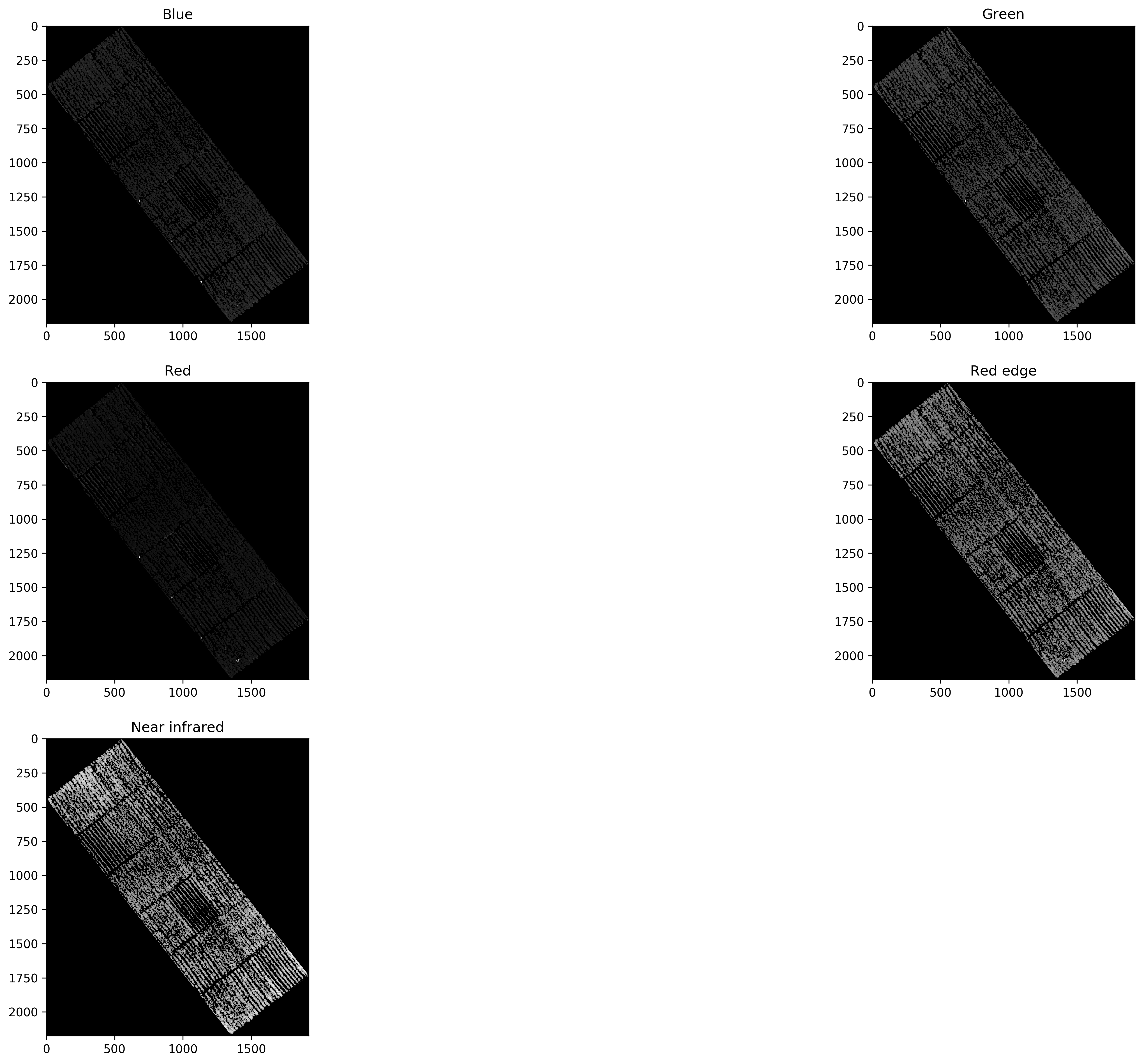
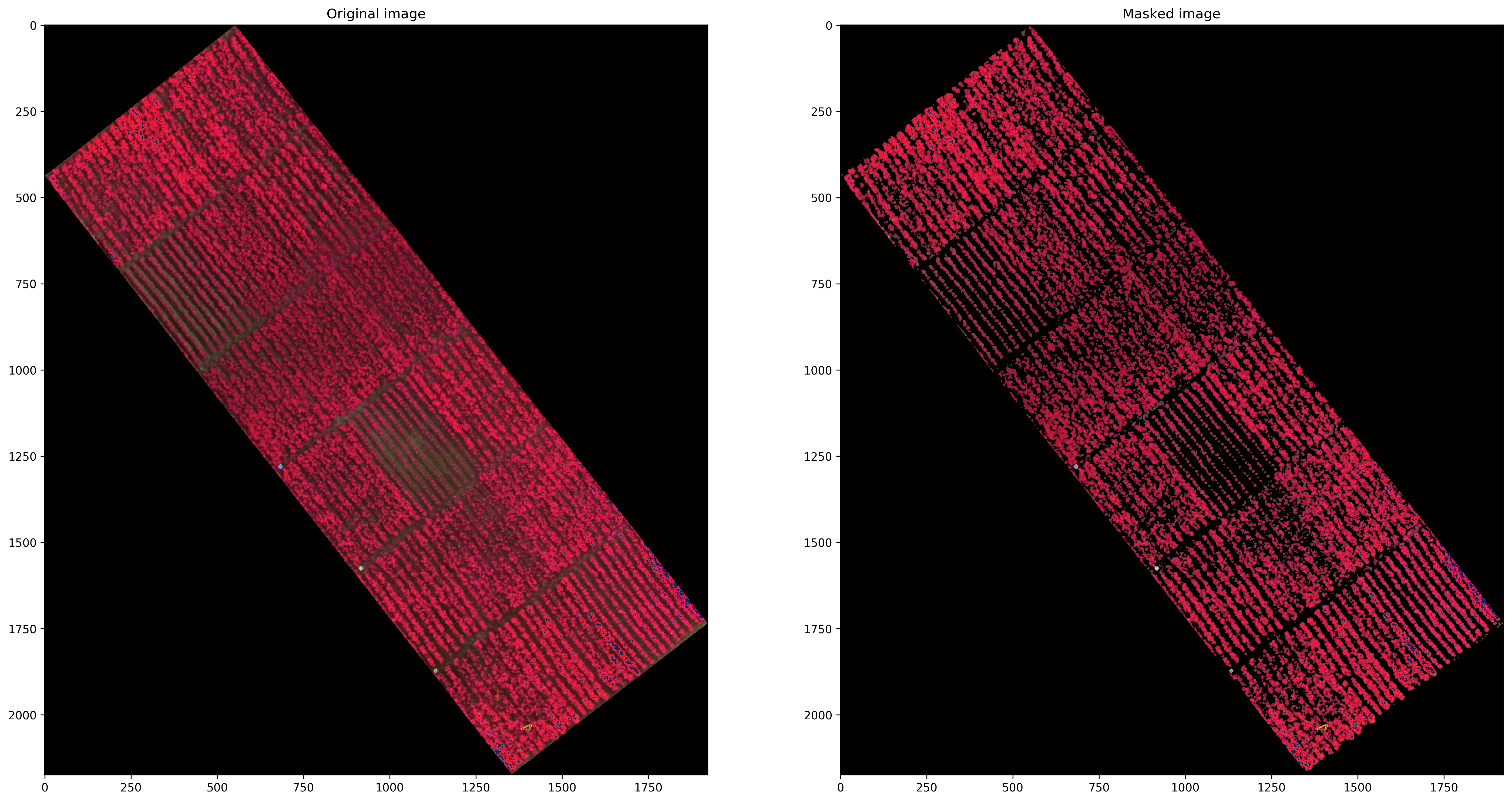
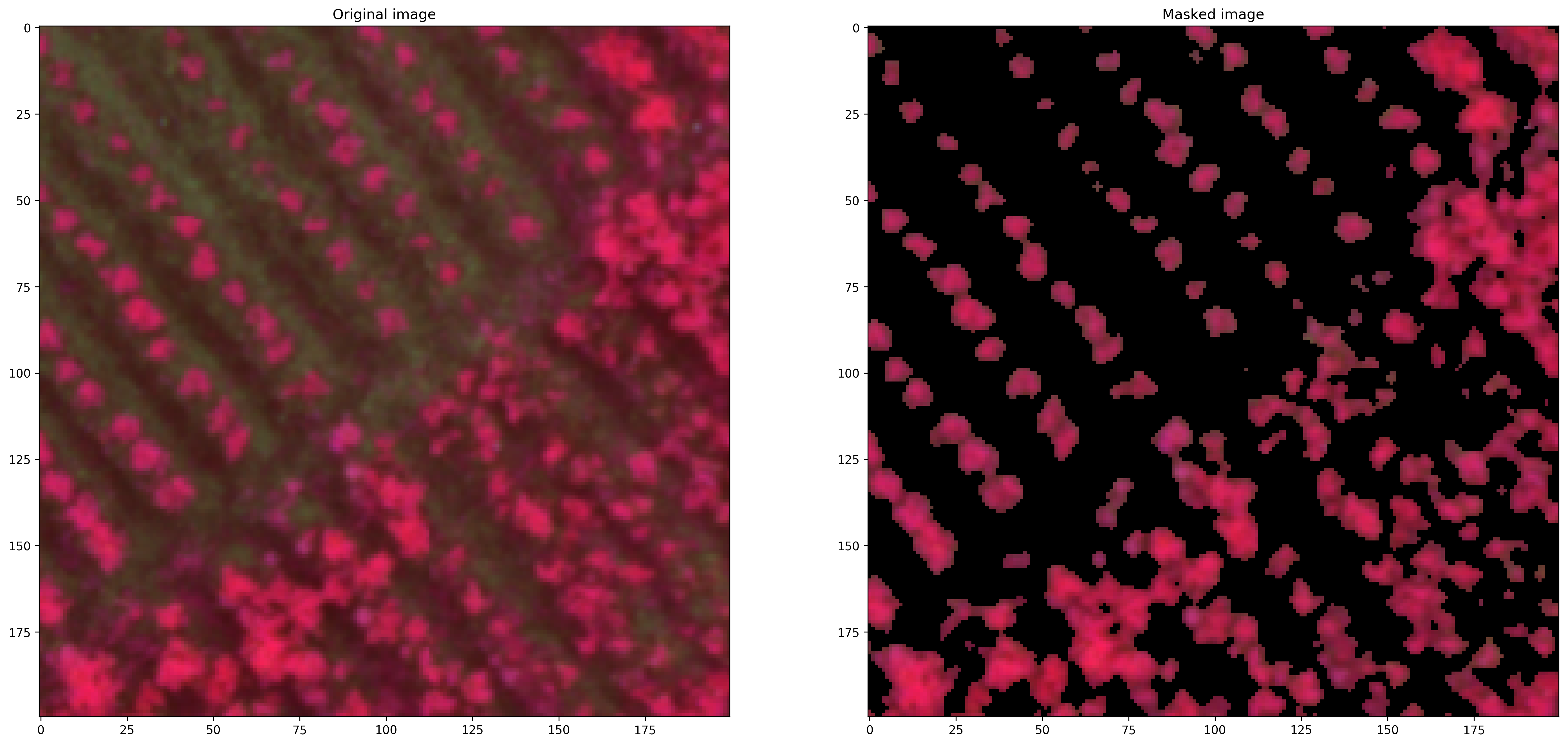
We can now create a false colour composition to improve the visualization of the background removing step. This was performed for visualisation purposes only:
# Contrast stretch function for enhance the bands
# Only for visualization purposes
def enhance_band(band, min_in= 0.1, max_in= 0.2):
    min_setup = 0.0
    max_setup = 1.0
    enhanced = (band-min_in)*(((max_setup-min_setup)/(max_in-min_in))+min_setup)
    return enhanced
NIR_IN = enhance_band(NIR, min_in= 0.0, max_in= (NIR.max()-0.10))
ROJO_IN = enhance_band(ROJO, min_in= 0.0, max_in= (ROJO.max()-0.08))
VERDE_IN = enhance_band(VERDE, min_in= 0.0, max_in= VERDE.max())

rgb = np.stack([NIR_IN,ROJO_IN,VERDE_IN], axis=2) #axis =2 so its shape is (M,N,3) otherwise doesn't work with plt. (M, N, 3): an image with RGB values (0-1 float or 0-255 int)
mask = cv2.cvtColor(filtered_mask, cv2.COLOR_GRAY2BGR) # So we can apply the mask
plantsImage = rgb*mask

plt.figure(1, dpi=300)
plt.subplots_adjust(left=0.0, right=3.0, bottom=0.0, top=3.0)
plt.subplot(121) ,plt.imshow(rgb),plt.title("Original image")
plt.subplot(122) ,plt.imshow(plantsImage),plt.title("Masked image")
plt.show()

plt.figure(2, dpi=300)
plt.subplots_adjust(left=0.0, right=3.0, bottom=0.0, top=3.0)
plt.subplot(121) ,plt.imshow(rgb[1250:1450,1100:1300]),plt.title("Original image")
plt.subplot(122) ,plt.imshow(plantsImage[1250:1450,1100:1300]),plt.title("Masked image")
plt.show()
Segmented bands to files
Now we proceed to save each of the segmented bands:
bands_out = np.stack([azul_seg,
                      verde_seg,
                      rojo_seg,
                      rededge_seg,
                      nir_seg],
                     axis=2)

band_names = {'M_2018-05-26_Corte_Seg_B1.tif':0,
              'M_2018-05-26_Corte_Seg_B2.tif':1,
             'M_2018-05-26_Corte_Seg_B3.tif':2,
             'M_2018-05-26_Corte_Seg_B4.tif':3,
             'M_2018-05-26_Corte_Seg_B5.tif':4
             }
dir_out = 'Raster/Segmented/'

for band_name in band_names:
    filename_output = dir_out + band_name
    index = band_names[band_name]
    x_size = ds.RasterXSize  # Raster xsize
    y_size = ds.RasterYSize  # Raster ysize
    driver = gdal.GetDriverByName('GTiff')
    arch = driver.Create(filename_output,x_size,y_size,1,gdal.GDT_Float32)
    arch.SetGeoTransform(geo_transform)
    arch.SetProjection(srs)
    arch.GetRasterBand(1).WriteArray(bands_out[:,:,index].astype(np.float32))
    del(arch)
    print("Band "+band_name+" exported")
Band M_2018-05-26_Corte_Seg_B4.tif exported
Band M_2018-05-26_Corte_Seg_B2.tif exported
Band M_2018-05-26_Corte_Seg_B1.tif exported
Band M_2018-05-26_Corte_Seg_B3.tif exported
Band M_2018-05-26_Corte_Seg_B5.tif exported
Classification of dataset: May 26, 2018
Loading segmented bands
rootdir = "Raster/Segmented"
# path to your model
path_model = "Data/Models/"
# path to your classification results
path_class = "Data/Class/"

ds_seg1 = gdal.Open('Raster/Segmented/M_2018-05-26_Corte_Seg_B1.tif')
ds_seg2 = gdal.Open('Raster/Segmented/M_2018-05-26_Corte_Seg_B2.tif')
ds_seg3 = gdal.Open('Raster/Segmented/M_2018-05-26_Corte_Seg_B3.tif')
ds_seg4 = gdal.Open('Raster/Segmented/M_2018-05-26_Corte_Seg_B4.tif')
ds_seg5 = gdal.Open('Raster/Segmented/M_2018-05-26_Corte_Seg_B5.tif')

Segmented_image = np.stack([ds_seg1.GetRasterBand(1).ReadAsArray(),
                           ds_seg2.GetRasterBand(1).ReadAsArray(),
                           ds_seg3.GetRasterBand(1).ReadAsArray(),
                           ds_seg4.GetRasterBand(1).ReadAsArray(),
                           ds_seg5.GetRasterBand(1).ReadAsArray()], axis=2)
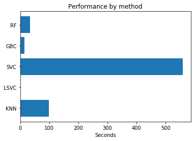
def plot_time(dt):
    fig, ax = plt.subplots()

    methods = ('RF', 'GBC', 'SVC', 'LSVC', 'KNN')
    y_pos = np.arange(len(methods))
    performance = dt

    ax.barh(y_pos, performance, align='center')
    ax.set_yticks(y_pos)
    ax.set_yticklabels(methods)
    ax.invert_yaxis()  # labels read top-to-bottom
    ax.set_xlabel('Seconds')
    ax.set_title('Performance by method')

    plt.show()

# declare a new function
def training(img_ds, path_model, path_class):

    img = img_ds.copy()

    ################### Random Forest Classifier ##########################
    # build your Random Forest Classifier
    # for more information: http://scikit-learn.org/stable/modules/generated/sklearn.ensemble.RandomForestClassifier.html
    ti_rf = time.time()
    # call your random forest model
    rf = path_model + "model_RF.pkl"
    clf = joblib.load(rf)

    # Classification of array and save as image (23 refers to the number of multitemporal NDVI bands in the stack)
    new_shape = (img.shape[0] * img.shape[1], img.shape[2])
    img_as_array = img[:, :, :23].reshape(new_shape)

    class_prediction = clf.predict(img_as_array)
    class_prediction = class_prediction.reshape(img[:, :, 0].shape)
    tf_rf = time.time()
    dt_rf = tf_rf - ti_rf

    #########################Gradient Boost Classifier#############################
    # alternatively you may try out a Gradient Boosting Classifier
    # It is much less RAM consuming and considers weak training data
    ti_gbc = time.time()

    GBC = path_model + "model_GBC.pkl"
    clf_GBC = joblib.load(GBC)

    # Classification of array and save as image (23 refers to the number of multitemporal NDVI bands in the stack)
    new_shape = (img.shape[0] * img.shape[1], img.shape[2])
    img_as_array = img[:, :, :23].reshape(new_shape)

    class_prediction_GBC = clf_GBC.predict(img_as_array)
    class_prediction_GBC = class_prediction_GBC.reshape(img[:, :, 0].shape)
    tf_gbc = time.time()
    dt_gbc = tf_gbc - ti_gbc

    #########################Support Vector Classifier#############################
    ti_svc = time.time()

    # call your SVC model
    svc = path_model + "model_svc.pkl"
    clf_svc = joblib.load(svc)

    # Classification of array and save as image (23 refers to the number of multitemporal NDVI bands in the stack)
    new_shape = (img.shape[0] * img.shape[1], img.shape[2])
    img_as_array = img[:, :, :23].reshape(new_shape)

    class_prediction_svc = clf_svc.predict(img_as_array)
    class_prediction_svc = class_prediction_svc.reshape(img[:, :, 0].shape)
    tf_svc = time.time()
    dt_svc = tf_svc - ti_svc
    #########################Linear Support Vector Classifier#############################
    ti_lsvc = time.time()

    # call your Linear SVC model
    lsvc = path_model + "model_lsvc.pkl"
    clf_lsvc = joblib.load(lsvc)

    # Classification of array and save as image (23 refers to the number of multitemporal NDVI bands in the stack)
    new_shape = (img.shape[0] * img.shape[1], img.shape[2])
    img_as_array = img[:, :, :23].reshape(new_shape)

    class_prediction_lsvc = clf_lsvc.predict(img_as_array)
    class_prediction_lsvc = class_prediction_lsvc.reshape(img[:, :, 0].shape)

    tf_lsvc = time.time()
    dt_lsvc = tf_lsvc - ti_lsvc
    ######################### KNN Classifier#############################
    ti_knn = time.time()

    # call your KNN model
    knn = path_model + "model_knn.pkl"
    clf_knn = joblib.load(knn)

    # Classification of array and save as image (23 refers to the number of multitemporal NDVI bands in the stack)
    new_shape = (img.shape[0] * img.shape[1], img.shape[2])
    img_as_array = img[:, :, :23].reshape(new_shape)

    class_prediction_knn = clf_knn.predict(img_as_array)
    class_prediction_knn = class_prediction_knn.reshape(img[:, :, 0].shape)

    tf_knn = time.time()
    dt_knn = tf_knn - ti_knn


    plot_time([dt_rf, dt_gbc, dt_svc, dt_lsvc,dt_knn])


    return class_prediction, class_prediction_GBC, class_prediction_svc, class_prediction_lsvc, class_prediction_knn
class_prediction, class_prediction_GBC, class_prediction_svc, class_prediction_lsvc, class_prediction_knn = training(Segmented_image, path_model, path_class)
[Parallel(n_jobs=2)]: Using backend ThreadingBackend with 2 concurrent workers.
[Parallel(n_jobs=2)]: Done  46 tasks      | elapsed:    3.1s
[Parallel(n_jobs=2)]: Done 196 tasks      | elapsed:   12.7s
[Parallel(n_jobs=2)]: Done 446 tasks      | elapsed:   29.7s
[Parallel(n_jobs=2)]: Done 500 out of 500 | elapsed:   33.2s finished
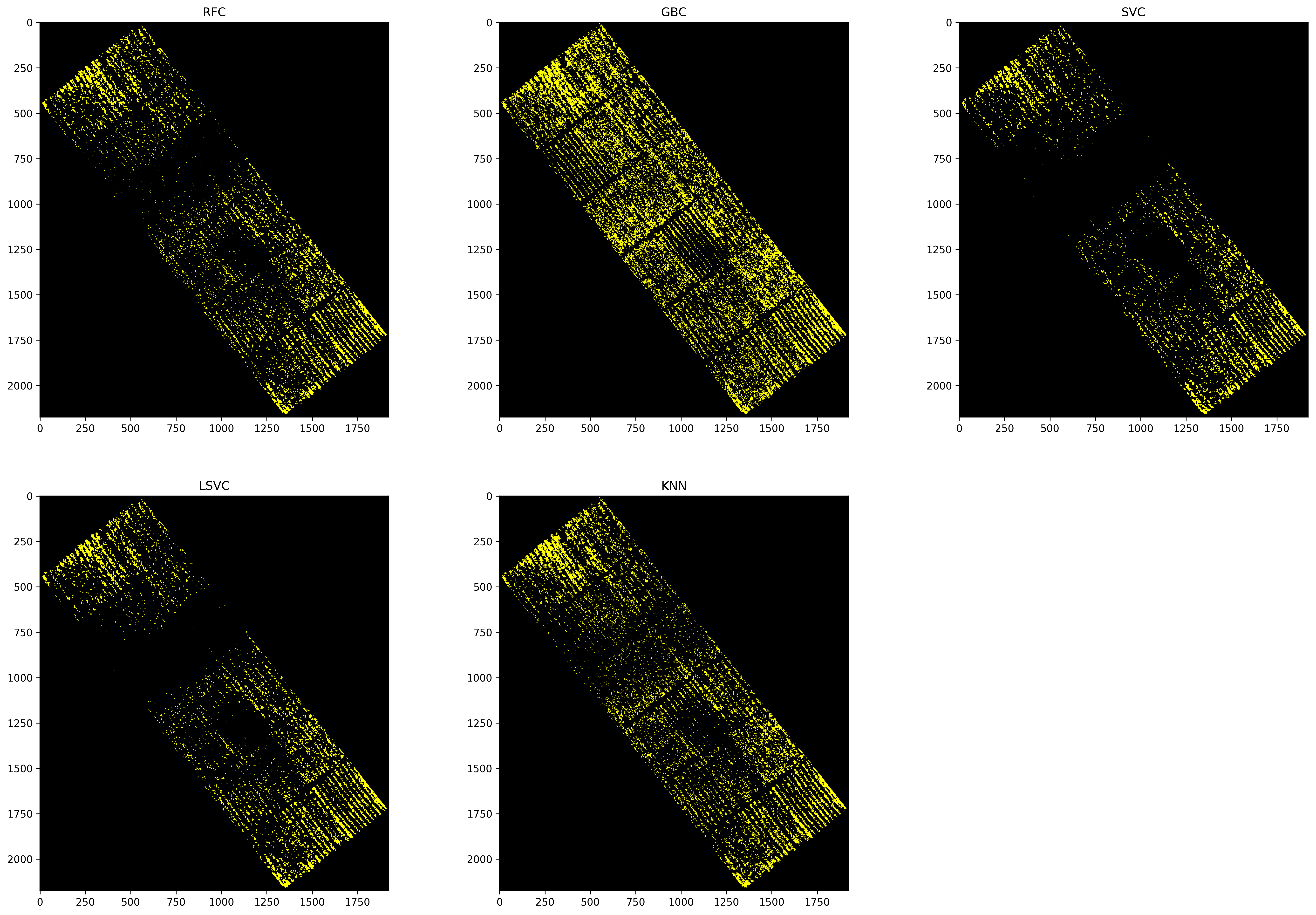
from matplotlib.colors import from_levels_and_colors
cmap, norm = from_levels_and_colors([0,0.5,1,2],['black','red','yellow'])

plt.figure(3, dpi=300)
plt.subplots_adjust(left=0.0, right=3.0, bottom=0.0, top=3.0)
plt.subplot(231) ,plt.imshow(class_prediction, cmap=cmap),plt.title('RFC')
plt.subplot(232) ,plt.imshow(class_prediction_GBC,cmap=cmap),plt.title('GBC')
plt.subplot(233) ,plt.imshow(class_prediction_svc,cmap=cmap),plt.title('SVC')
plt.subplot(234) ,plt.imshow(class_prediction_lsvc,cmap=cmap),plt.title('LSVC')
plt.subplot(235) ,plt.imshow(class_prediction_knn,cmap=cmap),plt.title('KNN')
plt.show()
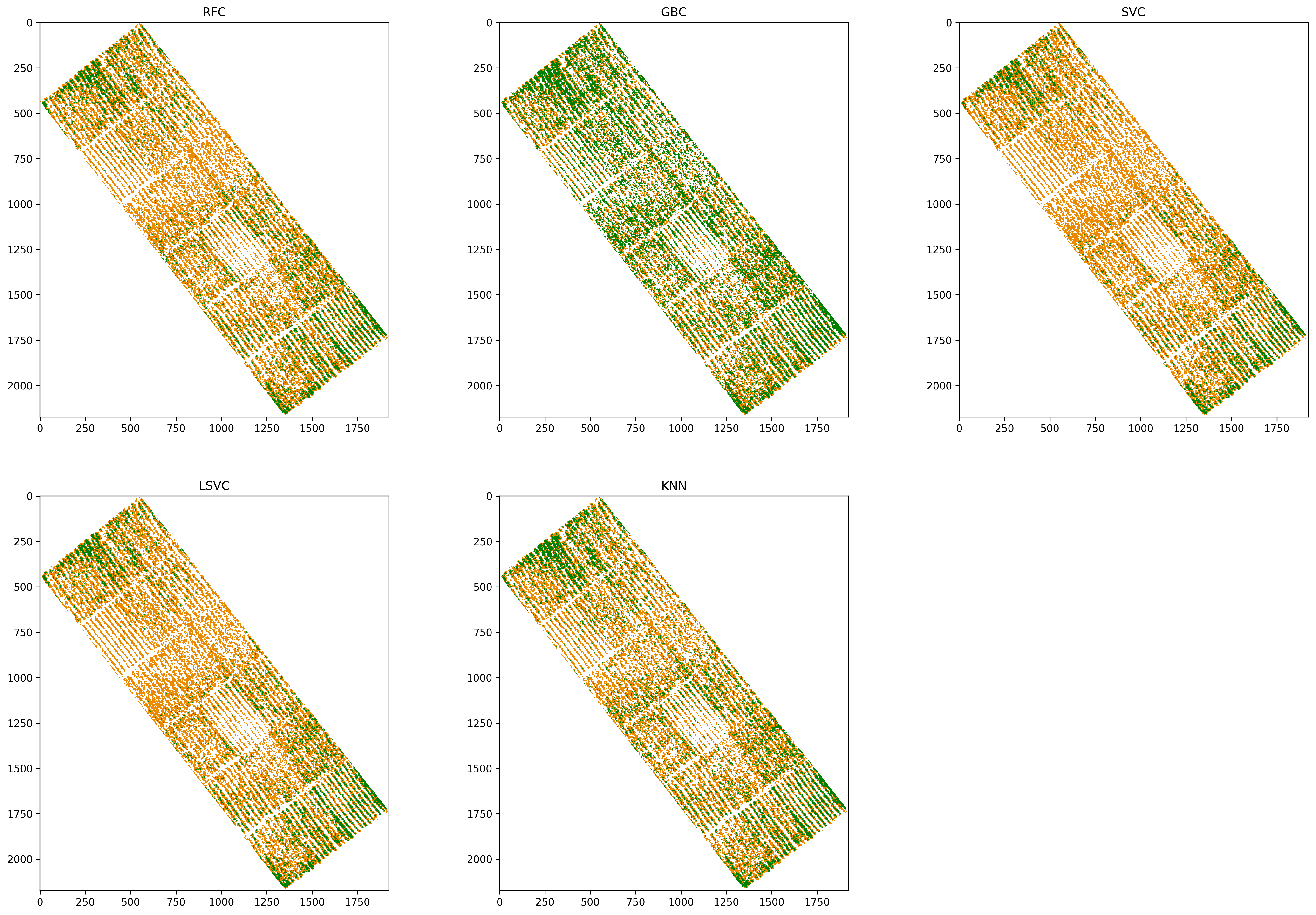
cmap, norm = from_levels_and_colors([0,0.5,1,2],['white','#EA8A00','green'])

rf_classification = class_prediction*filtered_mask
gbc_classification = class_prediction_GBC*filtered_mask
svc_classification = class_prediction_svc*filtered_mask
lsvc_classification = class_prediction_lsvc*filtered_mask
knn_classification = class_prediction_knn*filtered_mask

plt.figure(3, dpi=300)
plt.subplots_adjust(left=0.0, right=3.0, bottom=0.0, top=3.0)
plt.subplot(231) ,plt.imshow(rf_classification, cmap=cmap),plt.title('RFC')
plt.subplot(232) ,plt.imshow(gbc_classification,cmap=cmap),plt.title('GBC')
plt.subplot(233) ,plt.imshow(svc_classification,cmap=cmap),plt.title('SVC')
plt.subplot(234) ,plt.imshow(lsvc_classification,cmap=cmap),plt.title('LSVC')
plt.subplot(235) ,plt.imshow(knn_classification,cmap=cmap),plt.title('KNN')
plt.show()

plt.figure(1, dpi=300)
plt.subplots_adjust(left=0.0, right=3.0, bottom=0.0, top=3.0)
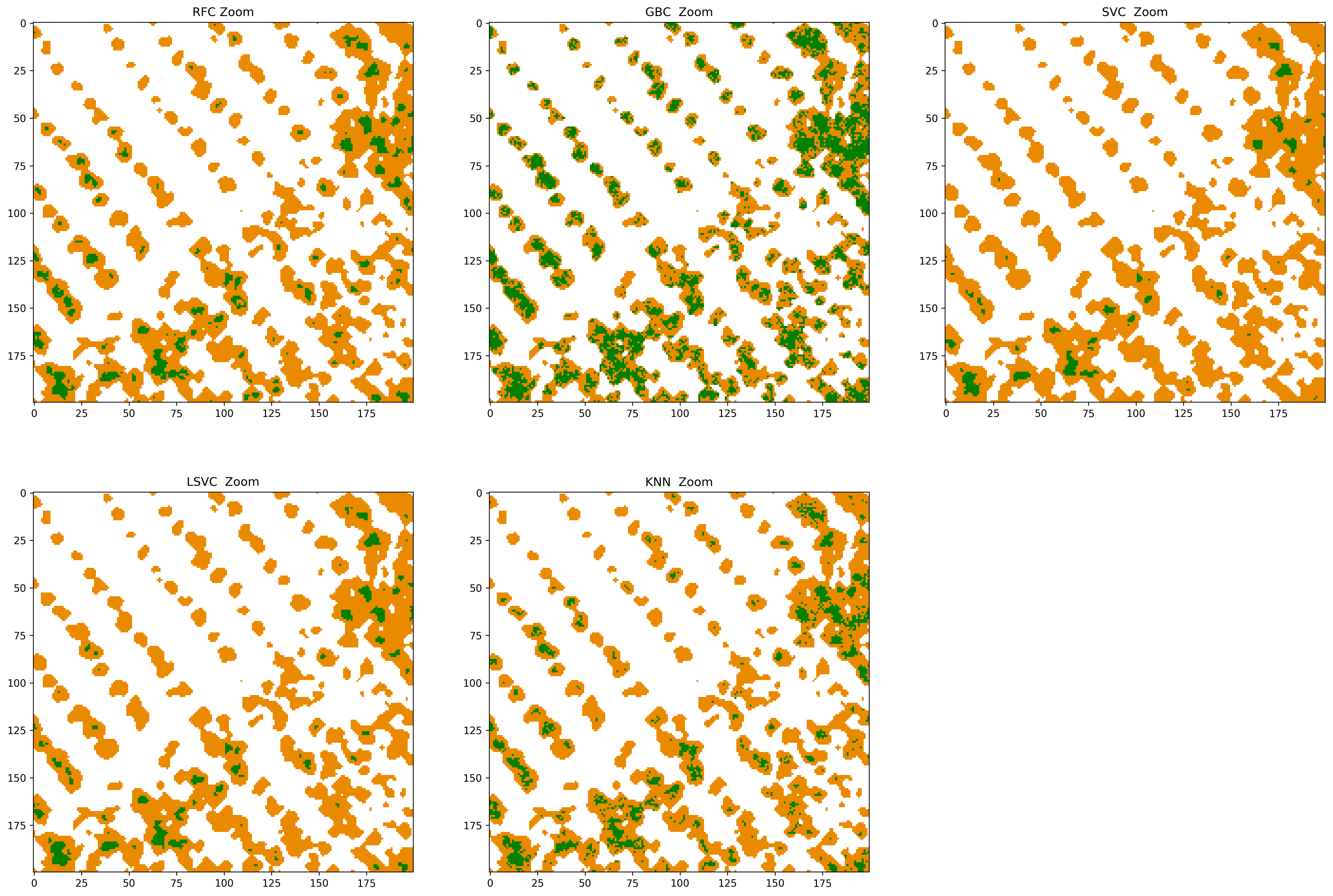
plt.subplot(231) ,plt.imshow(rf_classification[1250:1450,1100:1300], cmap=cmap),plt.title('RFC Zoom')
plt.subplot(232) ,plt.imshow(gbc_classification[1250:1450,1100:1300],cmap=cmap),plt.title('GBC  Zoom')
plt.subplot(233) ,plt.imshow(svc_classification[1250:1450,1100:1300],cmap=cmap),plt.title('SVC  Zoom')
plt.subplot(234) ,plt.imshow(lsvc_classification[1250:1450,1100:1300],cmap=cmap),plt.title('LSVC  Zoom')
plt.subplot(235) ,plt.imshow(knn_classification[1250:1450,1100:1300],cmap=cmap),plt.title('KNN  Zoom')
plt.show()
labels_class = np.unique(class_prediction[class_prediction > 0])
print('The classified data include {n} classes: {classes}'.format(n=labels_class.size, classes=labels_class))
The classified data include 2 classes: [1 2]
We can now save the classification results:
class_out = np.stack([rf_classification,
                      gbc_classification,
                      svc_classification,
                      lsvc_classification,
                     knn_classification],
                     axis=2)

class_names = {'Class_2018-05-26_RF.tif':0,
              'Class_2018-05-26_GBC.tif':1,
             'Class_2018-05-26_SVC.tif':2,
             'Class_2018-05-26_LSVC.tif':3,
             'Class_2018-05-26_KNN.tif':4
             }
dir_out = 'Resultados/Jupyter/'

for class_name in class_names:
    filename_output = dir_out + class_name
    index = class_names[class_name]
    x_size = ds.RasterXSize  # Raster xsize
    y_size = ds.RasterYSize  # Raster ysize
    driver = gdal.GetDriverByName('GTiff')
    arch = driver.Create(filename_output,x_size,y_size,1,gdal.GDT_Float32)
    arch.SetGeoTransform(geo_transform)
    arch.SetProjection(srs)
    arch.GetRasterBand(1).WriteArray(class_out[:,:,index].astype(np.float32))
    del(arch)
    print("Classification "+class_name+" exported")
Classification Class_2018-05-26_KNN.tif exported
Classification Class_2018-05-26_LSVC.tif exported
Classification Class_2018-05-26_GBC.tif exported
Classification Class_2018-05-26_SVC.tif exported
Classification Class_2018-05-26_RF.tif exported
Accuracy assessment of results
Loading ground reference
ds_ground_truth = gdal.Open('Validacion/Raster/Ground_truth_2018-05-26.tif')

# asignacion cada banda
ground_truth_array_raw = ds_ground_truth.GetRasterBand(1).ReadAsArray()
ground_truth_array = ground_truth_array_raw*filtered_mask
srs = ds_ground_truth.GetProjectionRef()
geo_transform = ds_ground_truth.GetGeoTransform()

cmap, norm = colors.from_levels_and_colors([0,0.5,1,2],['white','#EA8A00','green'])

plt.figure(1, dpi=300)
plt.subplots_adjust(left=0.0, right=3.0, bottom=0.0, top=3.0)
plt.subplot(121) ,plt.imshow(ground_truth_array, cmap=cmap),plt.title('Ground truth')
plt.subplot(122) ,plt.imshow(ground_truth_array[1250:1450,1100:1300], cmap=cmap),plt.title('Ground truth Zoom')
plt.show()
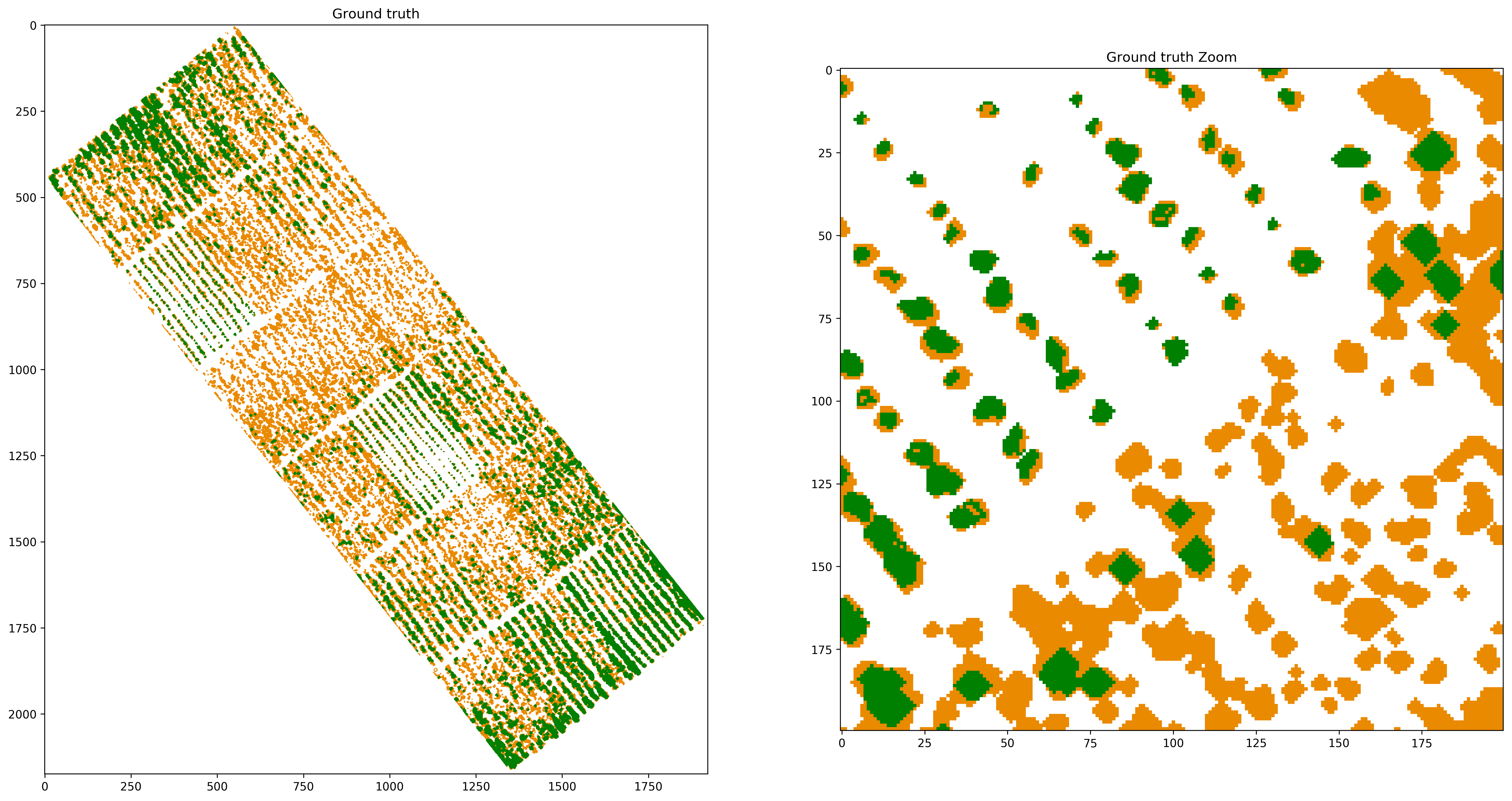
Ground truth details
def disease_info(array, geo_transform):
    unique, counts = np.unique(array[array!=0], return_counts=True)
    pix_width = geo_transform[1]
    pix_area = pix_width*pix_width

    lb_total_area = counts[0]*pix_area
    h_total_area = counts[1]*pix_area

    print("Late blight afected area: ", round(lb_total_area,2), "square meters")
    print("Healthy potato area: ", round(h_total_area,2), "square meters")
    print("Late blight vs Healthy potato area ratio: ", round(lb_total_area/h_total_area,2))
    print("Late blight area vs total area: ", round(lb_total_area/(lb_total_area+h_total_area),2))
    print("Healthy potato area vs total area: ", round(h_total_area/(lb_total_area+h_total_area),2))
disease_info(ground_truth_array, geo_transform)
Late blight afected area:  605.3 square meters
Healthy potato area:  337.79 square meters
Late blight vs Healthy potato area ratio:  1.79
Late blight area vs total area:  0.64
Healthy potato area vs total area:  0.36
Classification accuracy assessment
Because of the orientation of the experimental plot in relation to the north, and the segmentation of the orthomosaic to separate the plants of the background, we have a big area with zero values. The classification report from scikit-learn take those zeros into account, so global accuracy, macro avg and weighted avg in this report, in our case, may not represent accurately the metrics for the classification of late blight affected plants and healthy potato plants.
y_true = ground_truth_array.ravel()
target_names = ['0', 'Late blight', 'Healthy']

y_pred_rf = rf_classification.ravel()


print(classification_report(y_true, y_pred_rf, target_names=target_names))
              precision    recall  f1-score   support

           0       1.00      0.98      0.99   3407985
 Late blight       0.69      0.93      0.80    494491
     Healthy       0.82      0.52      0.64    275952

    accuracy                           0.94   4178428
   macro avg       0.84      0.81      0.81   4178428
weighted avg       0.95      0.94      0.94   4178428
Since the scikit report takes zeros into account as a class, we must create a function that allows us to calculate thematic accuracy metrics from the confusion matrix.
def corr_metrics(y_true, y_pred):
    cm = confusion_matrix(y_true,y_pred)
    lbc = cm[1]
    hp = cm[2]
    tp = float(lbc[1])
    fn = float(lbc[2])
    fp = float(hp[1])
    tn = float(hp[2])
    tot = tp+fp+fn+tn

    cm_c = pd.DataFrame(np.array([
        [tp, fp, tp+fp],
        [fn, tn, fn+tn],
        [tp+fn, fp+tn, tp+fp+fn+tn]
        ]),
        columns=['Actual - Late blight plants', 'Actual - Healthy plants', 'Total'],
        index =['Predicted - Late blight plants','Predicted - Healthy plants', 'Total'])
    ### ACC
    ACC = (tp + tn)/(tp + tn + fp + fn)
    ### MCC
    mcc_a = tp * tn - fp * fn
    mcc_b = math.sqrt((tp + fp) * (tp + fn) * (tn + fp) * (tn + fn))
    MCC = mcc_a / mcc_b
    ### Kappa ###
    ##Tp

    Pr_a_tp = (tp + tn)/tot
    Pr_A1_tp = (tp + fp)/tot
    Pr_B1_tp = (tp + fn)/tot
    PrA1B1_tp = Pr_A1_tp * Pr_B1_tp
    Pr_A2_tp = (fn + tn)/tot
    Pr_B2_tp = (fp + tn)/tot
    PrA2B2_tp = Pr_A2_tp * Pr_B2_tp
    Pr_e_tp = PrA1B1_tp + PrA2B2_tp

    kappa = (Pr_a_tp - Pr_e_tp)/(1 - Pr_e_tp)

    precision_tp = tp / (tp + fp)
    precision_tn = tn / (tn + fn)

    recall_tp = tp / (tp + fn)
    recall_tn = tn / (fp + tn)

    sup_tp = tp + fn
    sup_tn = fp + tn

    F_score_tp = 2*(tp)/(2*tp + fp + fn)
    F_score_tn = 2*(tn)/(2*tn + fp + fn)

    df_table = pd.DataFrame(np.array([
        [round(precision_tp,3), round(recall_tp,3), round(F_score_tp,3),sup_tp],
        [round(precision_tn,3), round(recall_tn,3), round(F_score_tn,3),sup_tn]
        ]),
        columns=['Precision', 'Recall', 'F1 score', 'Support'],
        index =['Late blight plants','Healthy plants'])
    #print('Accuraccy: ',round(ACC,2), '\nMCC: ', round(MCC,2))
    return df_table, cm_c, ACC, MCC, kappa
Random forest:
rf_table, cm_rf, rf_acc, rf_mcc, rf_kappa = corr_metrics(y_true, y_pred_rf)
cm_rf
| Actual - Late blight plants | Actual - Healthy plants | Total | |
|---|---|---|---|
| Predicted - Late blight plants | 462343.0 | 132425.0 | 594768.0 |
| Predicted - Healthy plants | 32148.0 | 143527.0 | 175675.0 |
| Total | 494491.0 | 275952.0 | 770443.0 |
rf_table
| Precision | Recall | F1 score | Support | |
|---|---|---|---|---|
| Late blight plants | 0.777 | 0.935 | 0.849 | 494491.0 |
| Healthy plants | 0.817 | 0.520 | 0.636 | 275952.0 |
print('Accuraccy: ',round(rf_acc,3),
      '\nMCC: ', round(rf_mcc,3),
      '\nKappa: ', round(rf_kappa,3))
Accuraccy:  0.786
MCC:  0.52
Kappa:  0.495
Disease details random forest
disease_info(rf_classification, geo_transform)
Late blight afected area:  814.67 square meters
Healthy potato area:  215.27 square meters
Late blight vs Healthy potato area ratio:  3.78
Late blight area vs total area:  0.79
Healthy potato area vs total area:  0.21
Gradient Boost Classifier
y_pred_gbc = gbc_classification.ravel()
gbc_table, gbc_cm, gbc_acc, gbc_mcc, gbc_kappa = corr_metrics(y_true, y_pred_gbc)
gbc_cm
| Actual - Late blight plants | Actual - Healthy plants | Total | |
|---|---|---|---|
| Predicted - Late blight plants | 280676.0 | 88581.0 | 369257.0 |
| Predicted - Healthy plants | 213815.0 | 187371.0 | 401186.0 |
| Total | 494491.0 | 275952.0 | 770443.0 |
gbc_table
| Precision | Recall | F1 score | Support | |
|---|---|---|---|---|
| Late blight plants | 0.760 | 0.568 | 0.650 | 494491.0 |
| Healthy plants | 0.467 | 0.679 | 0.553 | 275952.0 |
print('Accuraccy: ',round(gbc_acc,3),
      '\nMCC: ', round(gbc_mcc,3),
      '\nKappa: ', round(gbc_kappa,3))
Accuraccy:  0.608
MCC:  0.237
Kappa:  0.224
Disease details Gradient Boost Classifier
disease_info(gbc_classification, geo_transform)
Late blight afected area:  519.82 square meters
Healthy potato area:  510.11 square meters
Late blight vs Healthy potato area ratio:  1.02
Late blight area vs total area:  0.5
Healthy potato area vs total area:  0.5
Support Vector Classifier
y_pred_svc = svc_classification.ravel()
svc_table, svc_cm, svc_acc, svc_mcc, svc_kappa  = corr_metrics(y_true, y_pred_svc)
svc_cm
| Actual - Late blight plants | Actual - Healthy plants | Total | |
|---|---|---|---|
| Predicted - Late blight plants | 484622.0 | 151383.0 | 636005.0 |
| Predicted - Healthy plants | 9869.0 | 124569.0 | 134438.0 |
| Total | 494491.0 | 275952.0 | 770443.0 |
svc_table
| Precision | Recall | F1 score | Support | |
|---|---|---|---|---|
| Late blight plants | 0.762 | 0.980 | 0.857 | 494491.0 |
| Healthy plants | 0.927 | 0.451 | 0.607 | 275952.0 |
print('Accuraccy: ',round(svc_acc,3),
      '\nMCC: ', round(svc_mcc,3),
      '\nKappa: ', round(svc_kappa,3))
Accuraccy:  0.791
MCC:  0.545
Kappa:  0.487
Disease details Support Vector Classifier
disease_info(svc_classification, geo_transform)
Late blight afected area:  865.19 square meters
Healthy potato area:  164.75 square meters
Late blight vs Healthy potato area ratio:  5.25
Late blight area vs total area:  0.84
Healthy potato area vs total area:  0.16
Linear Support Vector Classifier
y_pred_lsvc = lsvc_classification.ravel()
lsvc_table, lsvc_cm, lsvc_acc, lsvc_mcc, lsvc_kappa  = corr_metrics(y_true, y_pred_lsvc)
lsvc_cm
| Actual - Late blight plants | Actual - Healthy plants | Total | |
|---|---|---|---|
| Predicted - Late blight plants | 477418.0 | 138036.0 | 615454.0 |
| Predicted - Healthy plants | 17073.0 | 137916.0 | 154989.0 |
| Total | 494491.0 | 275952.0 | 770443.0 |
lsvc_table
| Precision | Recall | F1 score | Support | |
|---|---|---|---|---|
| Late blight plants | 0.776 | 0.965 | 0.86 | 494491.0 |
| Healthy plants | 0.890 | 0.500 | 0.64 | 275952.0 |
print('Accuraccy: ',round(lsvc_acc,3),
      '\nMCC: ', round(lsvc_mcc,3),
      '\nKappa: ', round(lsvc_kappa,3))
Accuraccy:  0.799
MCC:  0.556
Kappa:  0.515
Disease details Linear Support Vector Classifier
disease_info(lsvc_classification, geo_transform)
Late blight afected area:  840.22 square meters
Healthy potato area:  189.72 square meters
Late blight vs Healthy potato area ratio:  4.43
Late blight area vs total area:  0.82
Healthy potato area vs total area:  0.18
K Neighbors Classifier
y_pred_knn = knn_classification.ravel()
knn_table, knn_cm, knn_acc, knn_mcc, knn_kappa  = corr_metrics(y_true, y_pred_knn)
knn_cm
| Actual - Late blight plants | Actual - Healthy plants | Total | |
|---|---|---|---|
| Predicted - Late blight plants | 416136.0 | 121061.0 | 537197.0 |
| Predicted - Healthy plants | 78355.0 | 154891.0 | 233246.0 |
| Total | 494491.0 | 275952.0 | 770443.0 |
knn_table
| Precision | Recall | F1 score | Support | |
|---|---|---|---|---|
| Late blight plants | 0.775 | 0.842 | 0.807 | 494491.0 |
| Healthy plants | 0.664 | 0.561 | 0.608 | 275952.0 |
print('Accuraccy: ',round(knn_acc,3),
      '\nMCC: ', round(knn_mcc,3),
      '\nKappa LB: ', round(knn_kappa,3))
Accuraccy:  0.741
MCC:  0.42
Kappa LB:  0.417
Disease details K-Neighbors Classifier
disease_info(knn_classification, geo_transform)
Late blight afected area:  743.04 square meters
Healthy potato area:  286.9 square meters
Late blight vs Healthy potato area ratio:  2.59
Late blight area vs total area:  0.72
Healthy potato area vs total area:  0.28
References
Glasbey, C.A., 1993. An Analysis of Histogram-Based Thresholding Algorithms.
Otsu, N., 1979. A Threshold Selection Method from Gray-Level Histograms. IEEE transactions on systems, man, and cybernetics 9, 62–66.arXiv:1011.1669v3.
Scikit-learn: Machine Learning in Python, Pedregosa et al., JMLR 12, pp. 2825-2830, 2011
Aknowlegments
We greatly acknowledge funding from National Geographic and Microsoft (‘AI for Earth’).